3 SNP-level parent-specific read counts to allele-specific transcription
3.1 Overview
This R tutorial follows quantification of SNP-level parent-specific mRNA-seq read counts and documents a statistical method for comparing allele-specific transcription between phenotypes in offspring derived from reciprocal crosses.
Sequencing data for this tutorial are described in Bresnahan et al., 2024, “Intragenomic conflict underlies extreme phenotypic plasticity in queen-worker caste determination in honey bees (Apis mellifera)”, bioRxiv. See the tutorial README for more details.
The honey bee gene annotations and the F1 SNPs intersecting honey bee genes generated in Section 2 are imported. SNPs are assigned to the longest transcript for each gene. SNPs intersecting \(n > 2\) genes or \(n = 2\) genes on the same strand are discarded, as it is impossible to assign SNP-level counts to genes with transcripts that overlap on the same strand. Additionally, SNPs within miRNA, tRNA, and repetitive pseudogenes are discarded as these are inappropriate for allele-specific analysis using short sequencing reads (for details, see: Wang & Clark, 2014, Heredity.)
The F2 read counts at F1 SNPs generated in Section 2 are imported. SNPs with \(n < 1\) count in any Lineage are discarded. In cases where the distance between SNPs is shorter than the average read length (and thus the read counts are exactly the same for both SNPs), one SNP is chosen at random. Finally, genes with \(n < 2\) SNPs are discarded, as this method requires at least two independent observations per gene for statistical analysis.
To adjust for differences in sequencing depth between libraries, library size factors are estimated and the read counts are normalized using the median of ratios normalization (MRN) method from DESeq2.
For each SNP, a Storer-Kim binomial exact test of two proportions is conducted using the MRN counts to test the hypothesis that the proportion of maternal and paternal read counts are statistically different.
A general linear mixed-effects model with interaction terms (GLIMMIX) is fit for each gene to assess the effects of Parent, Lineage, and their interaction on the raw read counts at each SNP, using the log of the library size factors as an offset to adjust for variation in sequencing depth between libraries. A Wald test is performed to assess the statistical significance of the effects.
For a gene to be considered as showing parent-of-origin or lineage-of-origin effects, all SNPs are required to exhibit the same directional bias in the Storer-Kim test, and a strictly parent-of-origin or lineage-of-origin effect in the GLIMMIX. To avoid identifying genes with parent-of-origin effects influenced by lineage-of-origin effects, or lineage-of-origin genes influenced by parent-of-origin effects, genes with a significant interaction effect are considered unbiased. Additionally, the proportions of Lineage A reads in samples with a Lineage B mother and Lineage A father (proportion 1, or p1), and the proportion of Lineage A reads in samples with a Lineage A mother and Lineage B father (p2), are subjected to a threshold test following methods described in Wang & Clark, 2014, Heredity.
3.2 Setup
3.2.1 Tutorial files
Download all files used in this tutorial here or via the command line:
3.2.2 Packages
Several CRAN packages are required for this tutorial. Use pacman to install those that are not already on your machine.
if (!require("pacman")) install.packages("pacman")
pacman::p_load("tidyverse", "plyr", "Rfast", "tryCatchLog",
               "lmerTest", "lme4", "car", "gridExtra",
               "doParallel", "ggpubr", "grid", "tagcloud",
               "ggprism")
This tutorial also uses a few Bioconductor packages. Use BiocManager to install them.
if (!require("BiocManager", quietly = TRUE))
    install.packages("BiocManager")

BiocManager::install(c("DESeq2","genomation","GenomicFeatures"))
Load all packages.
3.2.3 Custom functions
For efficiency, most of the code detailed throughout this tutorial has been compiled as custom functions, which are included in the project repository as AST-tutorial/AST_functions.R. These can be loaded into R during setup:
In this tutorial, each function will first be written explicitly to document how it works before demonstrating its use.
3.2.4 Sample metadata
Many of the custom functions described above reference the sample metadata, which must follow this specific format:
| sample.id | parent | block | phenotype | individual | lineage |
|---|---|---|---|---|---|
| PARENT_FILE | M or F | integer | character | FILE | A or B |
Note 1: For sample.id, PARENT_FILE corresponds to the file name suffix assigned to the SNP-level read count files generated in Section 2, with PARENT being the respective F1 genome to which the F2 mRNA-seq read FILE was aligned.
Note 2: lineage is synonymous with “maternal lineage” or “Cross” (as in Section 2). So, e.g., “lineage A” is synonymous with A-lineage mother x B-lineage father.
Sample metadata for the sequencing data described in Bresnahan et al., 2024, bioRxiv used in this tutorial has been included in the project repository as AST-tutorial/metadata.csv:
3.3 Generate sample x SNP:gene count matrix
3.3.1 Filter SNPs by transcript
The honey bee gene annotations saved as $AST-tutorial/{DIR_INDEX}/Amel_HAv3.1_genes.gff3 and the F1 SNPs intersecting honey bee genes saved as $AST-tutorial/{DIR_ANALYSIS}/SNPs_for_Analysis_Sorted.bed generated in Section 2 are imported. SNPs are assigned to the longest transcript for each gene, and SNPs within miRNA, tRNA, and repetitive pseudogenes and are discarded. A list of these genes has been included in the project repository as AST-tutorial/genelist_filter.csv.
# Load in filter list
filterlist <- read.csv("AST-tutorial/genelist_filter.csv",header=F)[,c(1)]

# Make txdb from the honey bee gene annotations
txdb <- makeTxDbFromGFF("AST-tutorial/INDEX/Amel_HAv3.1.gff")
transcripts <- transcripts(txdb)
Function: filter_SNPs
filter_SNPs <- function(SNP_gene_bed,exons,filterlist){
  ## SNP_gene_bed = bed file of SNPs intersecting genes
  ## exons = GRanges object containing exon regions
  ## filterlist = list of gene IDs to filter

  # Load in the SNPs BED file
  SNPs <- readBed(SNP_gene_bed)
  # Get SNPs that overlap with transcripts
  SNPs.exons <- findOverlaps(SNPs,exons)
  SNPs <- SNPs[queryHits(SNPs.exons)]
  SNPs <- data.frame(SNPs)[,c(1,2,7)]
  names(SNPs) <- c("chr","pos","SNP_gene")
  # Create SNP and geneID columns by splitting SNP_gene on ":"
  SNPs$SNP <- as.character(map(strsplit(SNPs$SNP_gene,split = ":"), 1))
  SNPs$geneID <- as.character(map(strsplit(SNPs$SNP_gene,split = ":"), 2))
  # Filter SNPs in genes within filterlist
  SNPs <- SNPs[!SNPs$geneID%in%filterlist,]
  # Delete any duplicate rows and clean up
  SNPs <- SNPs[!duplicated(SNPs),]
  rm(SNPs.exons)

  # Output
  return(SNPs)
}
# Execute
SNPs <- filter_SNPs("AST-tutorial/ANALYSIS_SETS/SNPs_for_Analysis_Sorted.bed",
transcripts,filterlist)
# Save output
write.csv(SNPs,"AST-tutorial/ANALYSIS/INTERMEDIATES/SNPs.csv",row.names=F)Example rows:
| chr | pos | SNP_gene | SNP | geneID |
|---|---|---|---|---|
| NC_037638.1 | 54752 | snp_99616:LOC107964061 | snp_99616 | LOC107964061 |
| NC_037638.1 | 91397 | snp_99617:LOC113219112 | snp_99617 | LOC113219112 |
| NC_037638.1 | 147183 | snp_99618:LOC726544 | snp_99618 | LOC726544 |
| NC_037638.1 | 148247 | snp_99619:LOC726544 | snp_99619 | LOC726544 |
| NC_037638.1 | 148360 | snp_99620:LOC726544 | snp_99620 | LOC726544 |
| NC_037638.1 | 148370 | snp_99621:LOC726544 | snp_99621 | LOC726544 |
3.3.2 Merge count files to matrix
The F2 read counts at F1 SNPs generated in Section 2 are imported. In cases where the distance between SNPs is shorter than the average read length (and thus the read counts are exactly the same for both SNPs), one SNP is chosen at random.
Function: make_ASE_counts_matrix
make_ASE_counts_matrix <- function(DIR_COUNTS,cores,SNPs){
  ## DIR_COUNTS = name of subdirectory containing count files
  ## cores = number of threads for parallel processing
  ## SNPs = dataframe generated by filter_SNPs2

  # Read in data
  ## List files ending in .txt in DIR_COUNTS
  SNP_counts <- data.frame(matrix(ncol=0,nrow=length(SNPs$SNP_gene)))
  SNP_counts$SNP_gene <- SNPs$SNP_gene
  files.counts <- list.files(path=DIR_COUNTS, pattern="*.txt",
                             full.names=TRUE, recursive=FALSE)
  ## Left join count files by SNP_ID:geneID
  for(i in 1:length(files.counts)){
    print(i)
    tmp.name <-  strsplit(strsplit(files.counts[[i]],
                                   split = "/")[[1]][length(strsplit(files.counts[[i]],
                                   split = "/")[[1]])],
                          split = "[.]")[[1]][1]
    if(tmp.name%in%metadata$sample.id){
      tmp <- read.table(files.counts[[i]],header=F)[,c(4,7)]
      names(tmp) <- c("SNP_gene",tmp.name)
      SNP_counts <- SNP_counts %>%
        left_join(tmp, by = c('SNP_gene' = 'SNP_gene'))
    }
  }
  rm(tmp,files.counts,tmp.name)

  # Clean up dataframe
  row.names(SNP_counts) <- SNP_counts$SNP_gene
  SNP_counts$SNP_gene <- NULL
  SNP_counts[is.na(SNP_counts)] <- 0
  SNP_counts$gene <- as.character(map(strsplit(row.names(SNP_counts), split = ":"), 2))

  # Remove duplicate rows within genes
  genelist <- unique(SNP_counts$gene)
  delete.rows <- list()
  ## Use DoParallel to perform loop operation in parallel
  registerDoParallel(cores=cores)
  delete.rows <- foreach(i=1:length(genelist)) %dopar% {
    tmp <- SNP_counts[SNP_counts$gene==genelist[i],]
    d <- row.names(tmp[duplicated(tmp),])
    delete.rows <- return(d)
  }
  SNP_counts <- SNP_counts[!row.names(SNP_counts)%in%unlist(delete.rows),]

  # Output
  return(SNP_counts)
}
# Execute
SNP_counts <- make_ASE_counts_matrix("AST-tutorial/COUNT",4,SNPs)
# Save output
write.csv(SNP_counts,"AST-tutorial/ANALYSIS/INTERMEDIATES/SNP_gene_counts.csv")Example rows:
| B3D_CMG0017_S9 | B3D_CMG0018_S10 | |
|---|---|---|
| snp_99616:LOC107964061 | 8 | 7 |
| snp_99617:LOC113219112 | 9 | 6 |
| snp_99618:LOC726544 | 7 | 11 |
| snp_99619:LOC726544 | 3 | 7 |
| snp_1:LOC726544 | 3 | 7 |
| snp_99623:LOC726544 | 3 | 8 |
3.4 Prepare sample x SNP:gene counts for analysis
3.4.1 Normalize by library size
In spite of every effort to standardize the library preparation and sequencing procedures, there are innumerable sources of between-sample variation that cannot be controlled for which will result in variation in sequencing depth between libraries. This is apparent here:
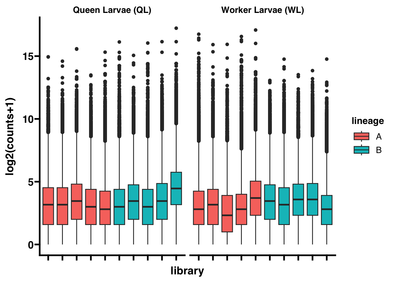
To adjust for differences in sequencing depth between libraries, library size factors are estimated and the read counts are normalized using the median of ratios normalization (MRN) method from DESeq2.
First, sum the parent-specific counts by library and estimate library size factors:
Function: calcSizeFactors
calcSizeFactors <- function(counts,mdata){
  ## counts = counts matrix generated by make_ASE_counts_matrix
  ## mdata = dataframe containing sample metadata

  # Merge parent-specific counts by library
  counts <- counts[,names(counts)%in%mdata$sample.id]
  counts_merged <- data.frame(matrix(ncol=0,nrow=length(row.names(counts))))
  samples <- unique(mdata$individual)
  for(i in 1:length(samples)){
    tmp <- counts[,names(counts)%in%mdata[mdata$individual==samples[i],"sample.id"]]
    tmp.merged <- rowSums(tmp)
    counts_merged <- cbind(counts_merged,tmp.merged)
  }
  names(counts_merged) <- samples
  mdata.merged <- mdata[,c("individual",
                           "phenotype",
                           "lineage")]
  mdata.merged <- mdata.merged[!duplicated(mdata.merged),]

  # Estimate library size factors using the median of ratios normalization method from DESeq2
  dds <- DESeqDataSetFromMatrix(countData = counts_merged, colData = mdata.merged,
                                design = ~ lineage + phenotype)
  dds <- estimateSizeFactors(dds)
  sizeFactors <- sizeFactors(dds)
  sF2meta <- data.frame(individual=names(sizeFactors))
  sF2meta$sF <- as.numeric(sizeFactors)
  sF2meta <- left_join(sF2meta,mdata[,c("individual",
                                        "sample.id")],
                       multiple = "all")
  sF2meta <- sF2meta[,c(3,2)]
  sF2meta <- sF2meta[match(names(counts), sF2meta$sample.id),]
  sFs <- sF2meta$sF
  names(sFs) <- sF2meta$sample.id

  # Output
  return(sFs)
}Second, perform the MRN method on the parent-specific counts using the library size factors calculated above.
Function: normalizeASReadCounts
normalizeASReadCounts <- function(counts,size_factors){
  ## counts = counts matrix generated by make_ASE_counts_matrix
  ## size_factors = array from calcSizeFactors

  # Normalize counts for each library by parent
  mdata <- metadata[metadata$sample.id%in%names(counts),]
  counts <- counts[,names(counts)%in%mdata$sample.id]
  as.dds <- DESeqDataSetFromMatrix(countData = counts, colData = mdata,
                                   design = ~ lineage+phenotype)
  sizeFactors(as.dds) = size_factors
  counts_normalized <- data.frame(counts(as.dds, normalized=TRUE))

  # Output
  return(counts_normalized)
}
# Execute
SNP_counts_normalized <- normalizeASReadCounts(SNP_counts,size_factors)
# Save output
write.csv(SNP_counts_normalized,"AST-tutorial/ANALYSIS/INTERMEDIATES/SNP_gene_counts_normalized.csv")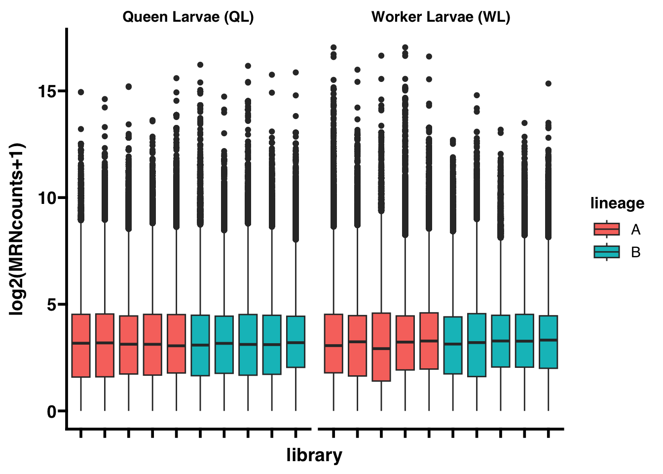
3.4.2 Split by phenotype and filter low count SNPs
Further filtering steps are performed after splitting the count matrix by phenotype. This is important as the set of transcribed genes is expected to vary between phenotypes. For the remainder of the tutorial, these phenotypes will be referred to in the code as “WL” and “QL” to match the sample metadata.
WL.IDs <- metadata[metadata$phenotype=="WL","sample.id"]
WL_counts_normalized <- SNP_counts_normalized[,names(SNP_counts_normalized)%in%WL.IDs]
WL_counts <- SNP_counts[row.names(SNP_counts)%in%row.names(WL_counts_normalized),
                                  names(SNP_counts)%in%WL.IDs]

QL.IDs <- metadata[metadata$phenotype=="QL","sample.id"]
QL_counts_normalized <- SNP_counts_normalized[,names(SNP_counts_normalized)%in%QL.IDs]
QL_counts <- SNP_counts[row.names(SNP_counts)%in%row.names(QL_counts_normalized),
                                names(SNP_counts)%in%QL.IDs]
SNPs with \(n < 1\) count in any Lineage are discarded. Finally, genes with \(n < 2\) SNPs are discarded, as this method requires at least two independent observations per gene for statistical analysis.
Note: here is where the utility of functions really becomes apparent. For the remainder of the tutorial, the same functions will be applied to the “WL” and “QL” count matrices.
Function: filter_counts
filter_counts <- function(counts,lcf){
  # counts = phenotype-specific counts matrix
  # lcf = low count filter threshold (integer)

  # Remove rows with < lcf counts counts by Lineage
  LA <- metadata[metadata$lineage=="A","sample.id"]
  LB <- metadata[metadata$lineage=="B","sample.id"]
  counts <- counts[rowSums(counts[,names(counts)%in%LA])>lcf,]
  counts <- counts[rowSums(counts[,names(counts)%in%LB])>lcf,]

  # Flag rows with greater than 10000 counts
  ## Different functions are used for SK tests with < and > 10000 counts for computational efficiency
  counts$SUM <- rowSums(counts)
  counts$SKrow <- F
  counts[counts$SUM<10000,"SKrow"] <- T
  counts$SUM <- NULL

  # Remove genes with < 2 SNPs
  counts$gene <- as.character(map(strsplit(row.names(counts), split = ":"), 2))
  genelist <- unique(counts$gene)
  delete.rows <- list()
  for(i in 1:length(genelist)){
    tmp <- counts[counts$gene==genelist[i],]
    tmp <- tmp[!duplicated(tmp),]
    if(length(row.names(tmp))<2){
      delete.rows <- append(delete.rows,genelist[i])
    }
  }
  counts <- counts[!counts$gene%in%unlist(delete.rows),]
  counts$gene <- NULL

  # Return filtered counts
  return(counts)
}
# Execute
WL_counts_normalized <- filter_counts(WL_counts_normalized,0)
WL_counts <- WL_counts[row.names(WL_counts)%in%row.names(WL_counts_normalized),]
QL_counts_normalized <- filter_counts(QL_counts_normalized,0)
QL_counts <- QL_counts[row.names(QL_counts)%in%row.names(QL_counts_normalized),]
# Save output
write.csv(WL_counts_normalized,"AST-tutorial/ANALYSIS/INTERMEDIATES/G53xY39_WL_counts_normalized.csv")
write.csv(WL_counts,"AST-tutorial/ANALYSIS/INTERMEDIATES/G53xY39_WL_counts.csv")
write.csv(QL_counts_normalized,"AST-tutorial/ANALYSIS/INTERMEDIATES/G53xY39_QL_counts_normalized.csv")
write.csv(QL_counts,"AST-tutorial/ANALYSIS/INTERMEDIATES/G53xY39_QL_counts.csv")3.5 Conduct statistical tests
The data are now ready for statistical analysis of allele-specific transcription. Storer-Kim, GLIMMIX, and threshold tests will be performed for each phenotype, separately, and then a Chi-squared test will be performed to compare the distribution of genes showing parent- and lineage-biased transcription between phenotypes.
3.5.1 SNP-level Storer-Kim (SK) binomial exact tests
For each SNP, a Storer-Kim binomial exact test of two proportions is conducted using the MRN counts to test the hypothesis that the proportion of maternal and paternal read counts are statistically different.
Function: twobinom
This test is performed using a modified version of the twobinom function from WRS2. For computational efficiency, the outer() command has been replaced with Rfast::Outer().
twobinom<-function(r1,n1,r2,n2,alpha=.05){
  # r1 = success in group 1
  # n1 = total in group 1
  # r2 = success in group 2
  # r2 = total in group 2
  n1p<-n1+1
  n2p<-n2+1
  n1m<-n1-1
  n2m<-n2-1
  q <- r1/n1
  p <- r2/n2
  if(is.na(q)){q <- 0}
  if(is.na(p)){p <- 0}
  chk<-abs(q-p)
  x<-c(0:n1)/n1
  y<-c(0:n2)/n2
  phat<-(r1+r2)/(n1+n2)
  m1<-t(Outer(x,y,"-"))
  m2<-matrix(1,n1p,n2p)
  flag<-(abs(m1)>=chk)
  m3<-m2*flag
  rm(m1,m2,flag)
  xv<-c(1:n1)
  yv<-c(1:n2)
  xv1<-n1-xv+1
  yv1<-n2-yv+1
  dis1<-c(1,pbeta(phat,xv,xv1))
  dis2<-c(1,pbeta(phat,yv,yv1))
  pd1<-NA
  pd2<-NA
  for(i in 1:n1){pd1[i]<-dis1[i]-dis1[i+1]}
  for(i in 1:n2){pd2[i]<-dis2[i]-dis2[i+1]}
  pd1[n1p]<-phat^n1
  pd2[n2p]<-phat^n2
  m4<-t(Outer(pd1,pd2,"*"))
  test<-sum(m3*m4)
  rm(m3,m4)
  list(p.value=test,p1=q,p2=p,est.dif=q-p)
}
Function: AST.SK
This is a wrapper function to perform the Storer-Kim test comparing the proportion of maternal to paternal read counts on each SNP in the count matrix. The Storer-Kim test has greater statistical power for low count observations, but is computationally expensive to perform and crashes when the total counts for a SNP are n > 10,000. Therefore, filter_counts flagged these rows, and AST.SK will instead perform a Fisher’s Exact test of two proportions, which is equivalent to a Storer-Kim test for high count observations. The test p-value is reported for each SNP.
Note: because this test is computationally expensive, executing AST.SK will take approximately 2hrs per 10,000 SNPs.
AST.SK <- function(counts,phenotype,cores){
  # counts = phenotype-specific counts matrix
  # phenotype = corresponding phenotype of counts
  # cores = # of threads for multithreaded search

  # Split data by pat and mat
  pat.exp <- counts[,metadata[metadata$parent%in%c("M")&
                                metadata$phenotype==phenotype,"sample.id"]]
  mat.exp <- counts[,metadata[metadata$parent%in%c("F")&
                                metadata$phenotype==phenotype,"sample.id"]]
  # Set up for DoParallel
  SKrows=counts$SKrow
  registerDoParallel(cores=cores)
  i.len=length(row.names(pat.exp))

  # For each row, conduct an SK test and return the p-value
  return.df <- foreach(i=1:i.len, .combine=rbind,
                       .export=ls(globalenv()),.packages="Rfast") %dopar% {
                         SNP_gene=row.names(pat.exp[i,])
                         p1.s=sum(pat.exp[i,])
                         p2.s=sum(mat.exp[i,])
                         p.o=sum(p1.s,p2.s)
                         if(SKrows[i]==T){
                           test=twobinom(r1=p1.s,n1=p.o,
                                         r2=p2.s,n2=p.o)$p.value
                         }else{
                           test=fisher.test(matrix(c(p1.s,p2.s,
                                                     p2.s,p1.s),ncol = 2))$p.value
                         }
                         return.append=data.frame(SNP_gene=SNP_gene,p=test)
                         return(return.append)
                       }
  return.df=return.df[match(row.names(pat.exp), return.df$SNP_gene),]

  # Return
  return(return.df)
}3.5.2 Gene-level general linear mixed models (GLIMMIX)
A general linear mixed-effects model with interaction terms (GLIMMIX) is fit for each gene to assess the effects of Parent, Lineage, and their interaction on the raw read counts at each SNP, using the log of the library size factors as an offset to adjust for variation in sequencing depth between libraries.
Function: AST.GLIMMIX
This is a wrapper function to fit a GLIMMIX for each gene in the count matrix and perform Wald tests to assess the statistical significance of the effects (parent, lineage, and their interaction). Wald test p-values are reported for each effect for each gene. Genes for which a model could not be fit due to errors are returned with a p-value of “1” for each effect.
AST.GLIMMIX <- function(counts,size_factors,cores){
  # counts = phenotype-specific counts matrix
  # phenotype = corresponding phenotype of counts
  # cores = # of threads for multithreaded search
  # size_factors = object from calcSizeFactors

  sizeFactors <- data.frame(t(size_factors[names(size_factors)%in%names(counts)]))
  sizeFactors <- gather(sizeFactors, sample.id, sizeFactor,
                        names(sizeFactors),factor_key=FALSE)
  counts$SNP_gene <- row.names(counts)
  counts$geneID <- as.character(unlist(map(strsplit(counts$SNP_gene,
                                                    split = ":"), 2)))
  genelist <- unique(counts$geneID)
  registerDoParallel(cores=cores)
  i.len <- length(genelist)

  df.out <- foreach(i=1:i.len,.combine=rbind) %dopar% {
    counts.sub <- counts[counts$geneID==genelist[i],]
    counts.sub$geneID <- NULL
    counts.sub <- gather(counts.sub, sample.id, count,
                         names(counts.sub), -SNP_gene, factor_key=TRUE)
    counts.sub <- join(counts.sub, metadata, by = "sample.id")
    counts.sub <- join(counts.sub,sizeFactors,by="sample.id")
    counts.sub$parent <- as.factor(str_sub(counts.sub$parent,-1,-1))
    counts.sub$SNP_gene <- as.factor(counts.sub$SNP_gene)
    counts.sub$lineage <- as.factor(counts.sub$lineage)
    counts.sub$individual <- as.factor(counts.sub$individual)
    testfail <- F
    test <- "null"
    tryCatchLog(test <- lmer(count~parent+lineage+parent*lineage+(1|SNP_gene)+
                               (1|individual)+offset(log(sizeFactor)),data=counts.sub),
                error = function(e) {testfail <- T})
    if(class(test)=="character"){testfail <- T}
    if(testfail==F){
      test <- summary(test)
      parent.p.list <- test[["coefficients"]][2,5]
      Lineage.p.list <- test[["coefficients"]][3,5]
      parent.Lineage.p.list <- test[["coefficients"]][4,5]
    }else{
      parent.p.list <- 1
      Lineage.p.list <- 1
      parent.Lineage.p.list <- 1
    }
    return(data.frame(ID=genelist[i],
                      parent.p=parent.p.list,
                      Lineage.p=Lineage.p.list,
                      parentXLineage.p=parent.Lineage.p.list))
  }
  return(df.out)
}3.6 Allele-specific transcription analysis
3.6.1 FDR correction and threshold tests
The False Discovery Rate (FDR) is now computed for the Storer-Kim and GLIMMIX (Wald) test results, requiring FDR < 0.05 for significance. For a gene to be considered as showing parent-of-origin or lineage-of-origin effects, all SNPs are required to exhibit the same directional bias (i.e., maternal or paternal) in the Storer-Kim test, and a strictly parent-of-origin or lineage-of-origin effect in the GLIMMIX. To avoid identifying genes with parent-of-origin effects influenced by lineage-of-origin effects, or lineage-of-origin genes influenced by parent-of-origin effects, genes with a significant interaction effect are considered unbiased.
Additionally, the proportions of Lineage A reads in samples with a Lineage B mother and Lineage A father (proportion 1, or p1), and the proportion of Lineage A reads in samples with a Lineage A mother and Lineage B father (p2), are subjected to a threshold test following methods described in Wang & Clark, 2014, Heredity. Specifically, thresholds of p1<0.4 and p2>0.6 are required for maternal bias, p1>0.6 and p2<0.4 for paternal bias, p1<0.4 and p2<0.4 for lineage B bias, and p1>0.6 and p2>0.6 for lineage A bias.
Note: remember here that lineage in metadata.csv is synonymous with “maternal lineage” or “Cross” (as in Section 2). So, e.g., “lineage A” is synonymous with A-lineage mother x B-lineage father.
Function: AST.Analysis
AST.Analysis <- function(counts,phenotype,SK,GLIMMIX){
  # counts = phenotype-specific count matrix
  # phenotype = corresponding phenotype of counts
  # SK = object from AST.SK
  # GLIMMIX = object from AST.GLIMMIX

  # Split count matrices by lineage and parent for plotting
  counts <- counts[,names(counts)%in%metadata$sample.id]
  p1.pat <- counts[,metadata[metadata$parent%in%c("M")&metadata$lineage=="B"&metadata$phenotype==phenotype,"sample.id"]]
  p1.mat <- counts[,metadata[metadata$parent%in%c("F")&metadata$lineage=="B"&metadata$phenotype==phenotype,"sample.id"]]
  p2.pat <- counts[,metadata[metadata$parent%in%c("M")&metadata$lineage=="A"&metadata$phenotype==phenotype,"sample.id"]]
  p2.mat <- counts[,metadata[metadata$parent%in%c("F")&metadata$lineage=="A"&metadata$phenotype==phenotype,"sample.id"]]

  # Set up a data.frame to plot p1 and p2 for each SNP
  p1.plot <- data.frame(rowSums(p1.pat)/(rowSums(p1.mat)+rowSums(p1.pat)))
  names(p1.plot) <- c("p1")
  p1.plot[is.nan(p1.plot$p1),"p1"] <- 0
  p2.plot <- data.frame(rowSums(p2.mat)/(rowSums(p2.mat)+rowSums(p2.pat)))
  names(p2.plot) <- c("p2")
  p2.plot[is.nan(p2.plot$p2),"p2"] <- 0
  plot <- cbind(p1.plot,p2.plot)

  # Join results of Storer-Kim tests
  plot <- plot[row.names(plot)%in%SK$SNP_gene,]
  plot$SK.p <- SK$p
  plot$SNP_gene <- row.names(plot)
  plot$gene <- as.character(map(strsplit(plot$SNP_gene, split = ":"), 2))

  # Reformat output from GLIMMMIX models
  GLIMMIX.biased <- data.frame(gene=GLIMMIX$ID,
                               parent.p=GLIMMIX$parent.p,
                               Lineage.p=GLIMMIX$Lineage.p,
                               parentXLineage.p=GLIMMIX$parentXLineage.p)

  # Correct for multiple testing
  plot$SK.padj <- p.adjust(plot$SK.p,"BH")
  plot$bias <- "NA"
  GLIMMIX$parent.padj <- p.adjust(GLIMMIX$parent.p,"BH")
  GLIMMIX$Lineage.padj <- p.adjust(GLIMMIX$Lineage.p,"BH")
  GLIMMIX$parentXLineage.padj <- p.adjust(GLIMMIX$parentXLineage.p,"BH")
  GLIMMIX.biased <- GLIMMIX[GLIMMIX$parent.padj<0.05|GLIMMIX$Lineage.padj<0.05,1]
  GLIMMIX.biased <- setdiff(GLIMMIX.biased,GLIMMIX[GLIMMIX$parentXLineage.padj<0.05,1])

  # For each gene, check whether all SNPs are biased in the same direction at established thresholds
  ## Genes with parentXLineage effects are flagged as unbiased
  for(i in 1:length(row.names(plot))){
    p <- plot[i,"SK.padj"]
    p1 <- plot[i,"p1"]
    p2 <- plot[i,"p2"]
    if(p<0.05&p1>0.6&p2<0.4){plot[i,"bias"] <- "pat"}
    if(p<0.05&p1<0.4&p2>0.6){plot[i,"bias"] <- "mat"}
    if(p<0.05&p1<0.4&p2<0.4){plot[i,"bias"] <- "Lineage B"}
    if(p<0.05&p1>0.6&p2>0.6){plot[i,"bias"] <- "Lineage A"}
  }
  biaslist <- data.frame(matrix(ncol=2,nrow=0))
  names(biaslist) <- c("gene","bias")
  genelist <- unique(plot$gene)
  for(i in 1:length(genelist)){
    tmp <- unique(plot[plot$gene==genelist[i],"bias"])
    if(length(tmp)>1){
      if(length(tmp)==2){
        if(any(tmp%in%"NA")){
          bias <- tmp[!tmp%in%"NA"]
        }else{bias <- "NA"}
      }else{
        bias <- "NA"
      }
    }else{bias <- tmp}
    biaslist <- rbind(biaslist,data.frame(gene=genelist[[i]], bias=bias))
  }
  plot <- plot %>% left_join(biaslist, by = c('gene' = 'gene'))
  names(plot)[c(7:8)] <- c("xbias","bias")
  plot$bias.plot <- "NA"
  for(i in 1:length(row.names(plot))){
    p1 <- plot$p1[i]
    p2 <- plot$p2[i]
    bias <- plot$bias[i]
    if(!bias=="NA"){
      if(bias=="pat"){if(p1>0.6&p2<0.4){plot[i,"bias.plot"]<- "pat"}}
      if(bias=="mat"){if(p1<0.4&p2>0.6){plot[i,"bias.plot"] <- "mat"}}
      if(bias=="Lineage B"){if(p1<0.4&p2<0.4){plot[i,"bias.plot"] <- "Lineage B"}}
      if(bias=="Lineage A"){if(p1>0.6&p2>0.6){plot[i,"bias.plot"] <- "Lineage A"}}
    }
  }
  plot[!plot$gene%in%GLIMMIX.biased,"bias.plot"] <- "NA"
  plot <- rbind(plot[plot$bias.plot%in%c("NA"),],
                plot[plot$bias.plot%in%c("mat", "Lineage A", "Lineage B", "pat"),])
  plot$bias.plot <- factor(plot$bias.plot,
                           levels = c("NA","mat", "Lineage A", "Lineage B", "pat"))

  # Return
  return(plot)
}
# Execute
WL.plot <- AST.Analysis(WL_counts_normalized,
"WL",metadata,WL.SK,WL.GLIMMIX)
QL.plot <- AST.Analysis(QL_counts_normalized,
"QL",metadata,QL.SK,QL.GLIMMIX)
# Save output
write.csv(WL.plot,"AST-tutorial/ANALYSIS/RESULTS/WLAST.csv",row.names=F)
write.csv(QL.plot,"AST-tutorial/ANALYSIS/RESULTS/QLAST.csv",row.names=F)The last three columns of a dataframe produced by AST.Analysis are informative of SNP and gene-level allelic bias:
xbias= SNP-level bias given 1) threshold test applied top1andp2, and 2) FDR-corrected SK-test p-value (SK.padj)bias= Gene-level bias given consistency ofxbiasvalue for each SNPbias.plot= Gene-level bias givenbiasand FDR-corrected GLIMMIX (Wald test) p-values. This is the reported value of allelic bias for each gene, and will be used to quantify the number of genes showing each category of allelic bias for performing Chi-squared tests.
3.6.2 Chi-squared tests
Finally, allele-specific transcription is compared between phenotypes. Specifically, Chi-squared tests are performed for each category of allelic bias to test the hypothesis that the distributions of biased and unbiased genes in each phenotype are statistically different.
For these tests, we will use the honey bee gene set (saved as ${DIR_INDEX}/Amel_HAv3.1_geneIDs.txt in Section 2) minus the genes in filterlist, as the “gene universe” - i.e., all possible genes that could have been expressed in these samples and tested for allele-specific transcription.
allgenes <- read.table("AST-tutorial/INDEX/Amel_HAv3.1_geneIDs.txt",header=F)[,1]
allgenes <- setdiff(allgenes,filterlist)
Function: AST.chisq
This is a wrapper function to perform these tests and format a table for plotting.
AST.chisq <- function(pheno1.label,pheno1.plot,
                      pheno2.label,pheno2.plot,
                      allgenes){
  # pheno1.label = label for phenotype 1
  # pheno1.plot = object from AST.Analysis
  # pheno2.label = label for phenotype 2
  # pheno2.plot = object from AST.Analysis
  # allgenes = list containing background set of genes

  # Collapse pheno plots by gene
  pheno1.plot <- pheno1.plot[,c("gene","bias.plot")]
  pheno1.plot <- pheno1.plot[!duplicated(pheno1.plot),]
  pheno2.plot <- pheno2.plot[,c("gene","bias.plot")]
  pheno2.plot <- pheno2.plot[!duplicated(pheno2.plot),]

  # Quantify genes in each category of bias and combine into a table
  gmid.df <- data.frame(
    Unresponsive=c(length(unique(pheno1.plot[pheno1.plot$bias.plot=="mat","gene"])),
                   length(unique(pheno1.plot[pheno1.plot$bias.plot=="Lineage A","gene"])),
                   length(unique(pheno1.plot[pheno1.plot$bias.plot=="Lineage B","gene"])),
                   length(unique(pheno1.plot[pheno1.plot$bias.plot=="pat","gene"]))),
    Bias=c("mat","Lineage A","Lineage B","pat"),
    Responsive=c(length(unique(pheno2.plot[pheno2.plot$bias.plot=="mat","gene"])),
                 length(unique(pheno2.plot[pheno2.plot$bias.plot=="Lineage A","gene"])),
                 length(unique(pheno2.plot[pheno2.plot$bias.plot=="Lineage B","gene"])),
                 length(unique(pheno2.plot[pheno2.plot$bias.plot=="pat","gene"]))))

  # Perform Chi-squared tests
  mat.test <- chisq.test(data.frame(Success=c(gmid.df[1,1],gmid.df[1,3]),
                                    Failure=c(length(allgenes)-gmid.df[1,1],
                                              length(allgenes)-gmid.df[1,3]),
                         row.names=c(pheno1.label,pheno2.label)),
                         correct=F)$p.value

  LineageA.test <- chisq.test(data.frame(Success=c(gmid.df[2,1],gmid.df[2,3]),
                                         Failure=c(length(allgenes)-gmid.df[2,1],
                                                   length(allgenes)-gmid.df[2,3]),                                           row.names=c(pheno1.label,pheno2.label)),
                              correct=F,simulate.p.value = TRUE)$p.value

  LineageB.test <- chisq.test(data.frame(Success=c(gmid.df[3,1],gmid.df[3,3]),
                                         Failure=c(length(allgenes)-gmid.df[3,1],
                                                   length(allgenes)-gmid.df[3,3]),
                              row.names=c(pheno1.label,pheno2.label)),
                              correct=F,simulate.p.value = TRUE)$p.value

  pat.test <- chisq.test(data.frame(Success=c(gmid.df[4,1],gmid.df[4,3]),
                                    Failure=c(length(allgenes)-gmid.df[4,1],
                                              length(allgenes)-gmid.df[4,3]),
                         row.names=c(pheno1.label,pheno2.label)),
                         correct=F)$p.value

  # Build table for plotting
  names(gmid.df) <- c(pheno1.label,"Bias",pheno2.label)
  gmid.df$p <- c(mat.test,LineageA.test,LineageB.test,pat.test)
  gmid.df <- gmid.df[,c(4,1,2,3)]
  nsrows <- row.names(gmid.df[gmid.df$p>0.05,])
  gmid.df$p <- formatC(gmid.df$p, format = "e", digits = 2)
  gmid.df[nsrows,"p"] <- "(ns)"
  gmid.df <- gmid.df[,c(2,3,4,1)]

  # Output
  return(gmid.df)
}We can see from this table that the QL group has more genes with paternal allele-biased transcription than the WL group, but the other categories of allelic bias are comparable between groups:
| WL | Bias | QL | p |
|---|---|---|---|
| 20 | mat | 11 | (ns) |
| 1 | Lineage A | 0 | (ns) |
| 3 | Lineage B | 2 | (ns) |
| 51 | pat | 92 | 5.84e-04 |
3.7 Data visualization
In this final section, the SNP-level counts are aggregated by gene to calculate and plot allelic transcription on p1 and p2. Data are plotted for each phenotype, separately, and then combined into a single plot separated by the Chi-squared test result table generated in the previous section.
First, reorder the data generated by AST.Analysis so that unbiased genes appear first:
WL.plot <- rbind(WL.plot[WL.plot$bias.plot%in%c("NA"),],
                           WL.plot[WL.plot$bias.plot%in%c(
                             "mat", "Lineage A", "Lineage B", "pat"),])
WL.plot$bias.plot <- factor(WL.plot$bias.plot,
                                      levels = c("NA","mat", "Lineage A",
                                                 "Lineage B", "pat"))

QL.plot <- rbind(QL.plot[QL.plot$bias.plot%in%c("NA"),],
                         QL.plot[QL.plot$bias.plot%in%c(
                           "mat", "Lineage A", "Lineage B", "pat"),])
QL.plot$bias.plot <- factor(QL.plot$bias.plot,
                                    levels = c("NA","mat", "Lineage A",
                                               "Lineage B", "pat"))
Function: AST.collapse
Next, use this function to collapse the data generated by AST.Analysis and calculate p1 and p2 by gene:
AST.collapse <- function(data.plot,data.counts,phenotype){
  # data.plot = object from AST.Analysis
  # data.counts = phenotype-specific counts matrix
  # phenotype = corresponding phenotype of data.plot and data.counts

  # Wrangle data
  data.counts <- data.counts[,names(data.counts)%in%metadata$sample.id]
  data.counts$SNP_gene <- row.names(data.counts)
  data <- data.plot %>%
    left_join(data.counts, by = c('SNP_gene' = 'SNP_gene'))
  genelist <- unique(data$gene)
  p1.mean <- list()
  p2.mean <- list()
  biaslist <- list()
  altbias <- list()

  # Collapse SNPs by gene
  for(i in 1:length(genelist)){
    tmp <- data[data$gene==genelist[i],]
    altbias[i] <- as.character(tmp$bias)[1]
    if(!any(tmp$bias=="NA") & length(tmp[!tmp$bias.plot=="NA","p1"])>0){
      tmp.sub <- tmp[!tmp$bias.plot=="NA",]
      # Split count matrices by Lineage and parent of origin for plotting
      p1.pat <- tmp.sub[,metadata[metadata$parent%in%c("M")&metadata$lineage=="B"&metadata$phenotype==phenotype,"sample.id"]]
      p1.mat <- tmp.sub[,metadata[metadata$parent%in%c("F")&metadata$lineage=="B"&metadata$phenotype==phenotype,"sample.id"]]
      p2.pat <- tmp.sub[,metadata[metadata$parent%in%c("M")&metadata$lineage=="A"&metadata$phenotype==phenotype,"sample.id"]]
      p2.mat <- tmp.sub[,metadata[metadata$parent%in%c("F")&metadata$lineage=="A"&metadata$phenotype==phenotype,"sample.id"]]
      p1.mean.x <- mean(sum(p1.pat)/(sum(p1.mat)+sum(p1.pat)))
      if(is.nan(p1.mean.x)){p1.mean.x <- 0}
      if(is.infinite(p1.mean.x)){p1.mean.x <- 1}
      p1.mean[i] <- p1.mean.x
      p2.mean.x <- mean(sum(p2.mat)/(sum(p2.mat)+sum(p2.pat)))
      if(is.nan(p2.mean.x)){p2.mean.x <- 0}
      if(is.infinite(p2.mean.x)){p2.mean.x <- 1}
      p2.mean[i] <- p2.mean.x
      biaslist[i] <- as.character(tmp.sub$bias.plot[1])
    }else{
      p1.mean[i] <- mean(tmp$p1)
      p2.mean[i] <- mean(tmp$p2)
      biaslist[i] <- "NA"}}
  return.data <- data.frame(gene=unlist(genelist),
                            bias.plot=unlist(biaslist),
                            p1=unlist(p1.mean),
                            p2=unlist(p2.mean),
                            altbias=unlist(altbias))
  return.data$bias.plot <- factor(return.data$bias.plot,
                                  levels = c("NA","mat", "Lineage A", "Lineage B", "pat"))
  return.data <- return.data[order(return.data$bias.plot),]

  # Output
  return(return.data)
}
# Execute
WL.collapse <- AST.collapse(WL.plot,WL_counts_normalized,"WL")
QL.collapse <- AST.collapse(QL.plot,QL_counts_normalized,"QL")
# Save output
write.csv(WL.collapse,"AST-tutorial/ANALYSIS/RESULTS/WLAST_collapse.csv",row.names=F)
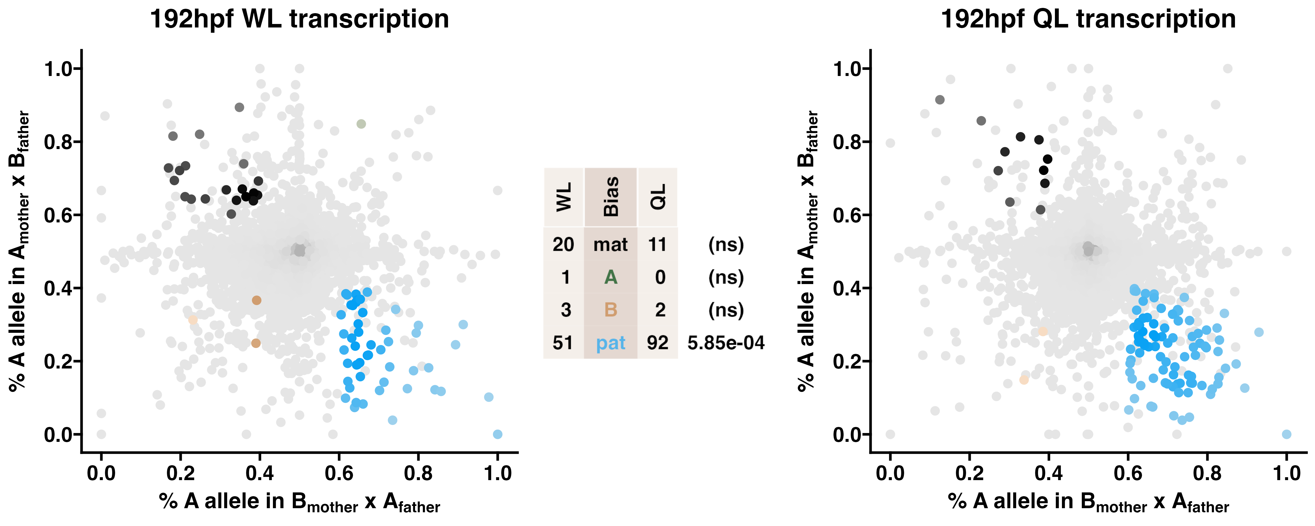
write.csv(QL.collapse,"AST-tutorial/ANALYSIS/RESULTS/QLAST_collapse.csv",row.names=F)Finally, generate scatter plots of allele-specific transcription joined by the table of Chi-squared test results.
Function: AST.scatter
This function generates a scatter plot of each gene by p1 and p2 for each phenotype. The points in these plots are assigned a color to represent its expression status: black is maternal, green is lineage A, gold is lineage B, blue is paternal, and grey is not significant. For consistency across studies, the colors for maternal, paternal, and unbiased genes are fixed, but the colors for each lineage can be customized. To help with visualizing the local density of points, each point is assigned its color value on a gradient between darker and lighter tones, indicating higher and lower local densities, respectively.
AST.scatter <- function(data,title,
                         LineageA.color.dark="#058762",LineageA.color.light="#4dc4a2",
                         LineageB.color.dark="#f7af05",LineageB.color.light="#f7ca60"){
  # data = object from AST.collapse
  # title = string, title of plot

  get_density <- function(x, y, ...){
    dens <- MASS::kde2d(x, y, ...)
    ix <- findInterval(x, dens$x)
    iy <- findInterval(y, dens$y)
    ii <- cbind(ix, iy)
    return(dens$z[ii])}

  data$bias.plot <- factor(data$bias.plot)
  biases <- levels(data$bias.plot)
  data$color <- NA
  for(i in 1:length(biases)){
    data.sub <- data[data$bias.plot==biases[i],]
    if(length(data.sub$gene)>2){
      density <- get_density(data.sub$p1, data.sub$p2, n = 100)
      if(biases[i]=="NA"){pal <- colorRampPalette(colors = c("grey90", "grey70"))(60)}
      if(biases[i]=="pat"){pal <- colorRampPalette(colors = c("#a1d2ed", "#02a0f5"))(60)}
      if(biases[i]=="mat"){pal <- colorRampPalette(colors = c("grey50", "black"))(60)}
      if(biases[i]=="Lineage A"){pal <- colorRampPalette(colors = c(LineageA.color.light,
                                                                    LineageA.color.dark))(60)}
      if(biases[i]=="Lineage B"){pal <- colorRampPalette(colors = c(LineageB.color.light,
                                                                    LineageB.color.dark))(60)}
      data[data$bias.plot==biases[i],"color"] <- smoothPalette(density,pal=pal)
    }
    if(length(data.sub$gene)<=2){
      if(biases[i]=="NA"){pal <- "grey90"}
      if(biases[i]=="pat"){pal <- "#a1d2ed"}
      if(biases[i]=="mat"){pal <- "grey50"}
      if(biases[i]=="Lineage A"){pal <- LineageA.color.light}
      if(biases[i]=="Lineage B"){pal <- LineageB.color.light}
      data[data$bias.plot==biases[i],"color"] <- pal
    }
  }
  data <- data[,c(3,4,6)]
  data <- data[!duplicated(data),]

  # Generate plot
  g <- ggplot(data, aes(x=p1, y=p2,
                        color=color)) +
    geom_point(size=3) + theme_prism() +
    xlab(expression(bold(paste("% A allele in ",B[mother],
                               " x ",A[father],sep="")))) +
    ylab(expression(bold(paste("% A allele in ",A[mother],
                               " x ",B[father],sep="")))) +
    ggtitle(title) +
    theme(text = element_text(size=18),
          plot.title = element_text(hjust = 0.5)) +
    guides(alpha=F, color=F) +
    scale_x_continuous(limits = c(0, 1), breaks = seq(0, 1, .2)) +
    scale_y_continuous(limits = c(0, 1), breaks = seq(0, 1, .2)) +
    scale_colour_identity()

  # Output
  return(g)
}
# Execute for WL
WL.scatter <- AST.scatter(WL.collapse,"192hpf WL transcription",
LineageA.color.dark="#427447",LineageA.color.light="#C1C9B5",
LineageB.color.dark="#d09d6f",LineageB.color.light="#f7dcc3")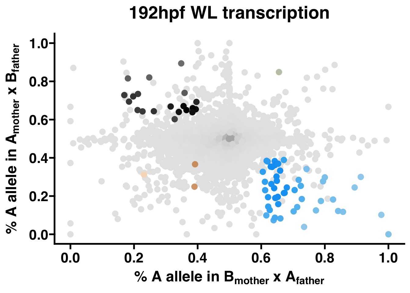
# Execute for QL
QL.scatter <- AST.scatter(QL.collapse,"192hpf QL transcription",
                          LineageA.color.dark="#427447",LineageA.color.light="#C1C9B5",
                          LineageB.color.dark="#d09d6f",LineageB.color.light="#f7dcc3")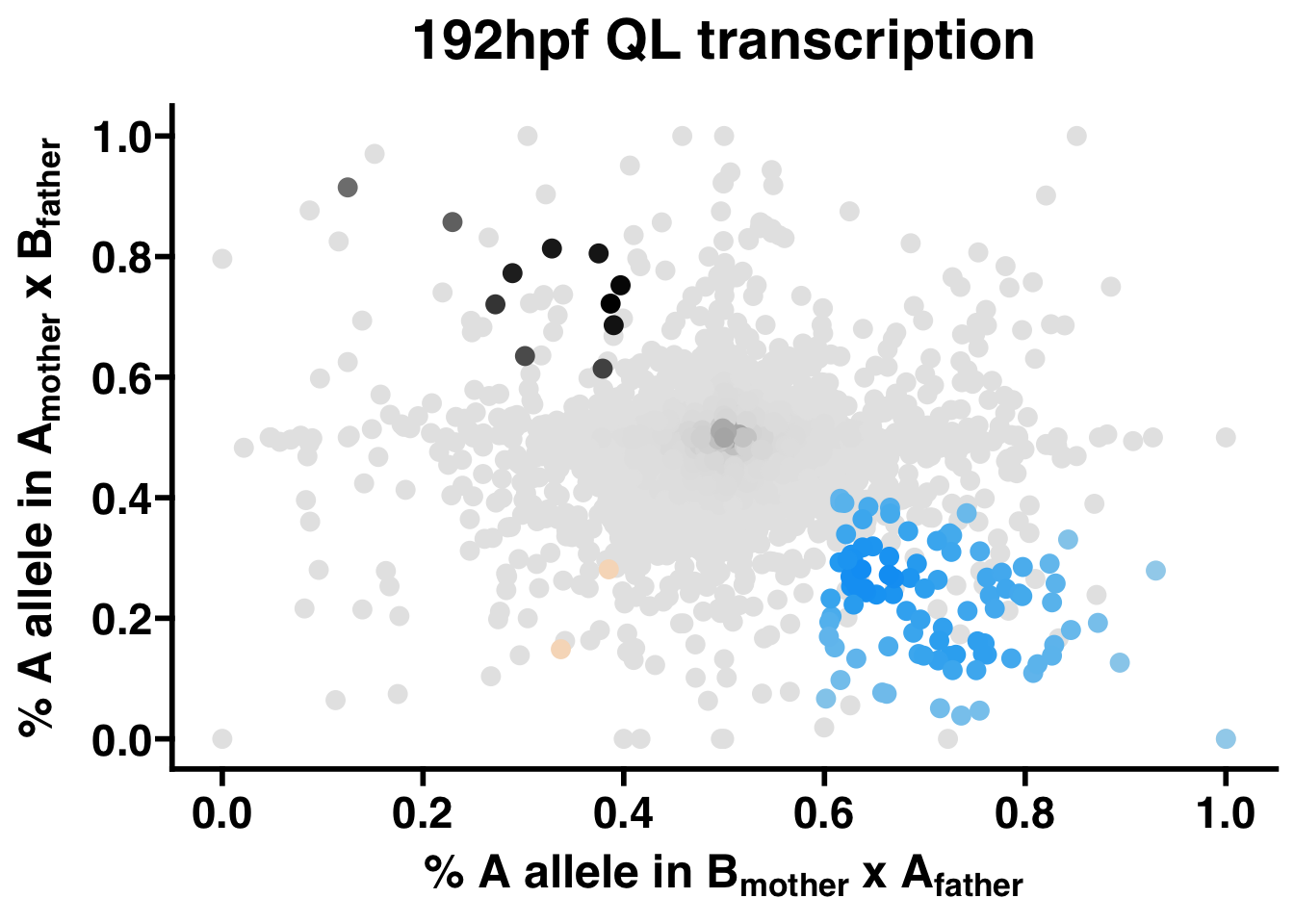
Function: AST.scatter.table
Plot the Chi-squared results table generated by AST.chisq.
AST.scatter.table <- function(chisq.df,
                              LineageA.color="#009e73",
                              LineageB.color="#e69f00"){
  # chisq.table = table generated by AST.chisq

  # Build table plot
  gmid.df <- chisq.df

  cols <- matrix("black", nrow(gmid.df), ncol(gmid.df))
  cols[1,2] <- "#000000"
  cols[2,2] <- LineageA.color
  cols[3,2] <- LineageB.color
  cols[4,2] <- "#56b4e9"

  ccols <- matrix("white", nrow(gmid.df), ncol(gmid.df))

  ccols[1:4,3] <- "#f4efea"
  ccols[1:4,1] <- "#f4efea"
  ccols[1:4,2] <- "#e4d8d1"

  cfonts <- matrix("bold", nrow(gmid.df), ncol(gmid.df))

  gmid.df[2,2] <- "A"
  gmid.df[3,2] <- "B"

  tt <- ttheme_default(core=list(fg_params = list(col = cols,
                                                  cex = 1,
                                                  fontface = cfonts),
                                 bg_params = list(col=NA, fill = ccols),
                                 padding.h=unit(2, "mm")),
                       rowhead=list(bg_params = list(col=NA)),
                       colhead=list(bg_params = list(fill =c("#f4efea",
                                                             "#e4d8d1",
                                                             "#f4efea",
                                                             "white")),
                                    fg_params = list(rot=90,
                                                     cex = 1,col=c("black",
                                                                   "black",
                                                                   "black",
                                                                   "white"))))

 # Generate plot
 gmid <- tableGrob(gmid.df, rows = NULL, theme=tt)

 # Output
 return(gmid)
}
# Execute
chisq.table <- AST.scatter.table(chisq.df,
LineageA.color="#427447",
LineageB.color="#d09d6f")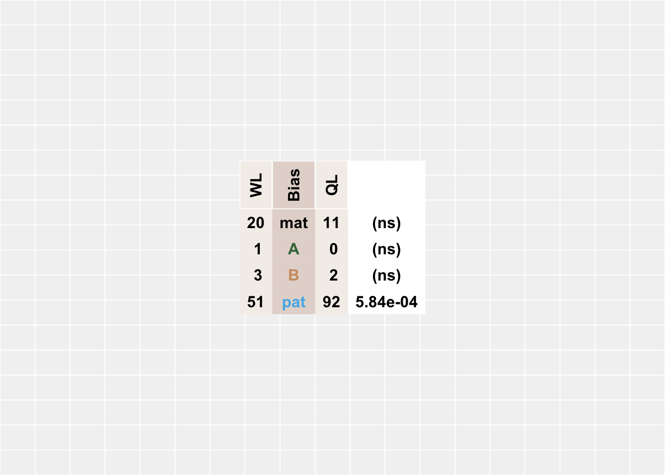
Combine the plots into a single figure to replicate Figure 4 from Bresnahan et al., 2024, “Intragenomic conflict underlies extreme phenotypic plasticity in queen-worker caste determination in honey bees (Apis mellifera)”, bioRxiv.
3.8 Session info
## R version 4.3.2 (2023-10-31)
## Platform: aarch64-apple-darwin20 (64-bit)
## Running under: macOS Ventura 13.1
##
## Matrix products: default
## BLAS:   /Library/Frameworks/R.framework/Versions/4.3-arm64/Resources/lib/libRblas.0.dylib
## LAPACK: /Library/Frameworks/R.framework/Versions/4.3-arm64/Resources/lib/libRlapack.dylib;  LAPACK version 3.11.0
##
## locale:
## [1] en_US.UTF-8/en_US.UTF-8/en_US.UTF-8/C/en_US.UTF-8/en_US.UTF-8
##
## time zone: America/New_York
## tzcode source: internal
##
## attached base packages:
##  [1] stats4    grid      parallel  stats     graphics  grDevices utils
##  [8] datasets  methods   base
##
## other attached packages:
##  [1] GenomicFeatures_1.54.4      AnnotationDbi_1.64.1
##  [3] genomation_1.34.0           DESeq2_1.42.1
##  [5] SummarizedExperiment_1.32.0 Biobase_2.62.0
##  [7] MatrixGenerics_1.14.0       matrixStats_1.1.0
##  [9] GenomicRanges_1.54.1        GenomeInfoDb_1.38.1
## [11] IRanges_2.36.0              S4Vectors_0.40.2
## [13] BiocGenerics_0.48.1         ggprism_1.0.4
## [15] tagcloud_0.6                ggpubr_0.6.0
## [17] doParallel_1.0.17           iterators_1.0.14
## [19] foreach_1.5.2               gridExtra_2.3
## [21] car_3.1-2                   carData_3.0-5
## [23] lmerTest_3.1-3              lme4_1.1-35.1
## [25] Matrix_1.6-3                tryCatchLog_1.3.1
## [27] Rfast_2.1.0                 RcppParallel_5.1.7
## [29] RcppZiggurat_0.1.6          Rcpp_1.0.11
## [31] plyr_1.8.9                  lubridate_1.9.3
## [33] forcats_1.0.0               stringr_1.5.1
## [35] dplyr_1.1.4                 purrr_1.0.2
## [37] readr_2.1.4                 tidyr_1.3.0
## [39] tibble_3.2.1                ggplot2_3.4.4
## [41] tidyverse_2.0.0             kableExtra_1.3.4
##
## loaded via a namespace (and not attached):
##   [1] splines_4.3.2            BiocIO_1.12.0            bitops_1.0-7
##   [4] filelock_1.0.2           XML_3.99-0.15            lifecycle_1.0.4
##   [7] rstatix_0.7.2            lattice_0.22-5           MASS_7.3-60
##  [10] backports_1.4.1          magrittr_2.0.3           sass_0.4.7
##  [13] rmarkdown_2.25           jquerylib_0.1.4          yaml_2.3.7
##  [16] plotrix_3.8-4            DBI_1.1.3                minqa_1.2.6
##  [19] RColorBrewer_1.1-3       abind_1.4-5              zlibbioc_1.48.0
##  [22] rvest_1.0.3              RCurl_1.98-1.13          rappdirs_0.3.3
##  [25] GenomeInfoDbData_1.2.11  svglite_2.1.2            codetools_0.2-19
##  [28] DelayedArray_0.28.0      xml2_1.3.5               tidyselect_1.2.0
##  [31] futile.logger_1.4.3      BiocFileCache_2.10.1     webshot_0.5.5
##  [34] GenomicAlignments_1.38.0 jsonlite_1.8.7           systemfonts_1.0.5
##  [37] tools_4.3.2              progress_1.2.2           glue_1.6.2
##  [40] SparseArray_1.2.2        xfun_0.41                withr_2.5.2
##  [43] numDeriv_2016.8-1.1      formatR_1.14             fastmap_1.1.1
##  [46] boot_1.3-28.1            fansi_1.0.5              digest_0.6.33
##  [49] timechange_0.2.0         R6_2.5.1                 seqPattern_1.34.0
##  [52] colorspace_2.1-0         biomaRt_2.58.2           RSQLite_2.3.3
##  [55] utf8_1.2.4               generics_0.1.3           data.table_1.14.8
##  [58] rtracklayer_1.62.0       prettyunits_1.2.0        httr_1.4.7
##  [61] S4Arrays_1.2.0           pkgconfig_2.0.3          gtable_0.3.4
##  [64] blob_1.2.4               impute_1.76.0            XVector_0.42.0
##  [67] htmltools_0.5.7          bookdown_0.38            scales_1.2.1
##  [70] png_0.1-8                knitr_1.45               lambda.r_1.2.4
##  [73] rstudioapi_0.15.0        tzdb_0.4.0               reshape2_1.4.4
##  [76] rjson_0.2.21             nlme_3.1-163             curl_5.1.0
##  [79] nloptr_2.0.3             cachem_1.0.8             KernSmooth_2.23-22
##  [82] restfulr_0.0.15          pillar_1.9.0             vctrs_0.6.4
##  [85] dbplyr_2.4.0             evaluate_0.23            cli_3.6.1
##  [88] locfit_1.5-9.9           compiler_4.3.2           futile.options_1.0.1
##  [91] Rsamtools_2.18.0         rlang_1.1.2              crayon_1.5.2
##  [94] ggsignif_0.6.4           stringi_1.8.2            viridisLite_0.4.2
##  [97] gridBase_0.4-7           BiocParallel_1.36.0      munsell_0.5.0
## [100] Biostrings_2.70.1        BSgenome_1.70.2          hms_1.1.3
## [103] bit64_4.0.5              KEGGREST_1.42.0          highr_0.10
## [106] broom_1.0.5              memoise_2.0.1            bslib_0.6.0
## [109] bit_4.0.5